PID in Advanced Ladder

Topic Menu

PID Control in Horner PLC

Hands-on PID Turning on the Horner OCS

Home > View > Project Toolbox > PID Operations

PID Elements in Advanced Ladder

PID stands for Proportional, Integral, Derivative. PID control provides a continuous variation of output within a control loop feedback mechanism to accurately control the process, removing oscillation and increasing process efficiency. Cscape provides two (2) PID (Proportional/Integral/Derivative) elements: Independent and ISA. These two elements differ only in how the proportional gain (Kp) component effects CV output.

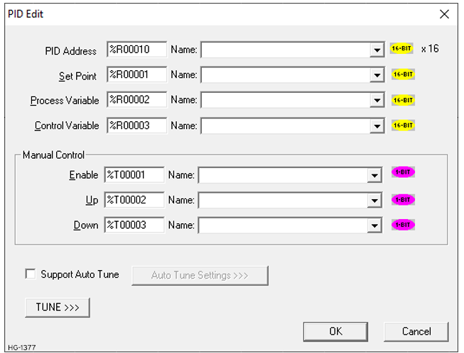
PID Address - Enter a Register or variable, this the base address of sixteen (16) consecutive WORD (16-bit) registers that the PID element uses to store its parameters. This value may NOT be a decimal constant.
Setpoint - Enter a Register or variable, this is the location of the User-defined Process Setpoint value. This value may NOT be a decimal constant.
Process Variable - Enter a Register or variable, this is the location (typically %AI) of the Process Variable value coming in from the process. This value may NOT be a decimal constant.
Control Variable - Enter a Register or Variable, this is the location (typically %AQ) of the Control Variable value going out to the process. This value may NOT be a decimal constant.
Manual Input - Enter a Register or variable for user-controlled Manual Input bit. This register is a Boolean (1-bit) register.
Up Input - Enter a Register or Variable for user-controlled UP Input bit. This register is a Boolean (1-bit) register.
Down Input - Enter a Register or Variable for user-controlled DOWN Input bit. This register is a Boolean (1-bit) register.
Support Auto Tune - Select this option to enable support for auto tune PID.
Auto Tune Settings - Click on this button to set the registers and options used for auto tuning. See PID Auto Tune for more information.
Tune>>> - Click on the TUNE>>> button to invoke the PID Element Tuning dialog.

Register Usage

PID element requires an array of Sixteen (16) WORD (16-bit) registers. These will presumably be of type %R. This is called the Reference Array.

Offset	Parameter	Units	Range	Description
0	Sample Period	10 mS	0 to 65535	The shortest time, in 10mS increments, allowed between PID solutions.
1	Deadband +	PV Counts	0 to 32000	Defines the Upper Deadband limits in terms of PV counts. Set both to 0 (zero) if no dead band is required.
2	Deadband -	PV Counts	-32000 to 0	Defines the Lower Deadband limits in terms of PV counts. Set both to 0 (zero) if no dead band is required.
3	Proportional Gain (Kp)	Percent	0 to 327.67%	Sets the Proportional Gain (Kp) factor in terms of percent. 100 sets unity gain (gain of 1).
4	Derivative Gain (Kd)	10 mS	0 to 327.67 seconds	Entered as a time with a resolution of 10 mS. In the PID equation this has the effect: Kd * delta Error / dt.
5	Integral Rate (Ki)	Repeats per 1000 second	0 to 32.767 repeats per second	Entered as a number of repeats per second -- effectively the integration rate. In the PID equation this has the effect: Ki * Error * dt
6	CV Bias	CV Counts	-32000 to +32000	Number of CV counts added to the output before the rate and amplitude clamps.
7	CV Upper Clamp	CV Counts	32000 to +32000	Number of CV Counts that represent the highest and lowest value for CV. CV Upper Clamp must be more positive the CV Lower Clamp
8	CV Lower Clamp	CV Counts	-32000 to +32000
9	Minimum Slew Time	Seconds of full travel	0 to 32000 seconds to move 32000 CV counts	Determines how fast the CV value can change.
10	Config Word	N/A	N/A	Internal Use - Do not modify this value.
11	Manual Command	CV Counts	Tracks CV in Auto mode; sets CV in Manual Mode.	In the Automatic mode this register tracks the CV value. In the Manual Mode, this register contains the value that is output to the CV within the clamp and slew limits.
12	Internal SP	Used by OCS	N/A	Tracks SP Input value
13	Internal PV	Used by OCS	N/A	Tracks PV Input value
14	Internal CV	Used by OCS	N/A	Tracks CV Output value
15	Cycle Time	Seconds	N/A	Cycle Time for PWM in Seconds

Each PID element must use a distinctly separate Reference Array, even if the values are identical to an existing PID element. There can be no overlapping of PID elements.

Registers at offset 0 through 9 must be configured before the PID element is used. This is most easily done using the Tune features of the Cscape PID Element Configuration. These registers can, however, be manipulate by the ladder program as well.

Return to the Top: PID in Advanced Ladder

PID Independent (with and without Auto Tuning)

The elements are configured from the PID Independent Element Configuration dialog.

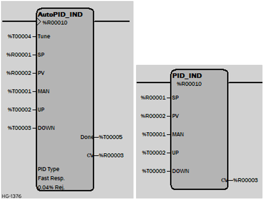
The element uses an array of Sixteen (16) WORD (16-bit) registers, presumably type %R. This is known as the Reference Array (see below).In operation, when the element receives power, and the Manual Input does not receive power, the element is placed in the Automatic Mode. The element first determines if it's sample time period has elapsed. If the time period has elapsed, the PID algorithm is solved and the Control Variable (CV) is updated.

If power is applied to the element and power is also applied to the Manual input, the element operates in the Manual Mode. The Control Variable (CV) is updated using the value in the Manual Command Parameter in the reference array. If the UP or DOWN inputs are also active, the CV count is incremented or decremented by one CV count on every PID solution.

In either manual or automatic modes, the CV Output value is limited by both the CV Clamp Value and the CV Slew Limit value. If the Internal CV value exceeds either clamp value or the rate of change of the Internal CV exceeds the Slew Limit, the value of CV Output is clamped at the limit. CV Output moves away from the clamp value at such time as the Internal CV values drops below the clamp or the slew rate drops below the CV Slew Rate limit. This provides an anti-windup protection and bump less transfer between automatic and manual modes.

If the element receives power, it solves the PID equation only if the sample time period has been exceeded. Setting the Sample Time Period to 0 indicates that the equation is to be solved every time the element is enabled, but in no case the element executes faster than once every 10 milliseconds. For example, if the OCS scan time is 9 milliseconds, and Sample Time Period is set to 0 (zero), the element executes once every other scan, or 18 mS. The element can not execute in the first scan, because the 10 millisecond minimum limit has not been met. The element can not again execute until the next scan, 9 milliseconds later.

When the tune input goes high, the PID functions starts the auto tune process. If power is removed from the tune input before the tuning process is complete, the auto tune procedure is aborted. Note to eliminate the anti-windup feature of the PID loop, the integral term is set to zero when the autotune starts. When the auto tune process completes, the done output goes high and the PID loop continues running with the newly calculated coefficients.

Equation

Independent PID:

CVout = (Kp * Error) + (Ki * Error * dt) + (Kd * Derivative) + CVBias

Where:

dt = Internal elapsed time clock - previous elapsed time clock

Derivative = (Error - previous Error)/dt

--or--

Derivative = (pv - previous PV)/dt

[User selectable during configuration].

Ti = Integral time

Td = Derivative time

In the Independent PID the Kp value is used alone while in the ISA PID, the Kp value is used to factor both the Ki and Kd values. The Independent PID is the standard function, but the ISA PID is a bit easier to tune.

Return to the Top: PID in Advanced Ladder

PID ISA (with and without Auto Tuning)

The elements are configured from the PID ISA Element Configuration dialog.

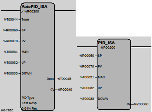
The difference between PID_IND and PID_ISA is only how the proportional gain (Kp) component effects CV output.

Equation

ISA PID:

CVout = Kp * (Error + (Error * dt / Ti) + (Td * Derivative)) + CVBias

Where:

dt = Internal elapsed time clock - previous elapsed time clock

Derivative = (Error - previous Error)/dt

--or--

Derivative = (pv - previous PV)/dt

[User selectable during configuration].

Ti = Integral time

Td = Derivative time

Return to the Top: PID in Advanced Ladder

PID Controls

PID Control in Horner PLC

Hands-on PID Turning on the Horner OCS

In a typical industrial process, one often wants to control some parameter of a process such as heat or pressure. This can be done in an open loop fashion:

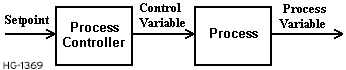
In such a system, the Process Controller accepts some value from the user. This value is called the Setpoint. The Process Controller then generates a value to be sent to the process called the Control Variable. The desired parameter is the Process Variable, which changes in response to the value sent by the Process Controller. The problem with this system is that there is no way for the Process Controller to determine if the process is actually producing the proper Process Variable. The Process Controller must assume that the process completes it's job quickly and accurately. In many cases, this is sufficient.

But these assumptions are often incorrect or inaccurate. The process may simply be inaccurate in itself. For example, a heater can be told to produce 350 degrees but actually produces 400 degrees. There is also the possibility that changes in the process itself may produce errors. For example, adding hot or cold materials to a process certainly changes the temperature of the process. Any change in the system that produces a change in the Process Variable is called a disruption. A disruption can be caused by purposely changing the Setpoint or can be a side effect of some process activity like adding or subtracting material from the process. The control system needs to respond equally well to disruptions at either point and to both positive-going and negative-going changes.

Most process control systems use feedback. This is called a closed loop system. In these systems, the Process Variable is measured, and that value returned to the Process Controller:

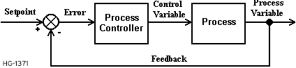
Such a process can respond to both changes in the Setpoint value and to changes in the process or load. Change the setpoint, and the controller tries to drive the process to the new value. Change the value of the Process Variable and the controller tries to drive the process back to the Setpoint value.

The question in this situation is, "What do we do with the feedback?" In most applications, the feedback is subtracted from the setpoint to produce a value called Error. The magnitude of Error is determined by the difference between the Setpoint value and the Process Variable value. For example, a simple temperature controller might accept a setpoint of 350 degrees. The Process Variable measures 200 degrees. Therefore, the Error value is 150 degrees.

The first thought is to add the Error to the Setpoint, and use this value to drive the process towards the desired value in less time. In the above example, adding the 350 degrees Setpoint and the 150 degrees Error attempts to drive the process to 500 degrees, which would have the effect of causing the process to heat up faster. On the next reading, the Process Variable is found to be 250 degrees making the Error 100 degrees. The controller adds the Error to the Setpoint and tries to drive the process towards 450 degrees. Further readings find the process warmer. The Error is smaller, and the process moves slowly towards the final temperature.

The problem with such an arrangement is that the process can change too much before the changes from the controller can affect it. In the above example, the process might actually go to 400 or more degrees before the controller can bring it back down. Conversely, the temperature can drop significantly before the controller makes the necessary changes.

PID Terminology

Some terms need to be defined in order for a meaningful discussion of PID performance to be presented.

PID - Proportional, Integral, Derivative Control (PID) - An intelligent I/O module or program instruction providing automation closed-loop operation of process control loops. For each loop, this module or instruction can perform proportional control and optionally integral control, derivative control, or both.

Proportional Control – Causes an output signal to change as a direct ratio of the error signal variation.
Integral Control – Causes an output signal to change as a function of the integer or the error signal over the time duration.
Derivative Control – Causes an output signal to change as a function of the rate or change of the error signal.

Setpoint - In a feedback control loop, the commanded value of the variable being controlled. See SP below.

Control Variable - The output of a process controller (Proportional, Proportional/Integral, or Proportional/Integral/Derivative) used to "drive" the process towards the desired setpoint. See CV below.

Process Variable - The current actual value of a process -- temperature, pressure, flow rate, etc. See PV below.

Bias - A component often added to PID equations that adds a constant offset to the final value.. BIAS - generally used with Proportional-only controls, and is set to 0 if Integral Control action is used.

K - Process Open Loop Gain as figured by PVstep / CVstep.

Kp - Proportional Gain. This is the amount of Error Value that is ultimately fed back to the system. Sometimes called Controller Gain (Kc).

Ki - Integral Gain. Actually a time period defining how often the Error is "integrated". Faster time is the equivalent of higher gain in the Integral portion.

Kd - Derivative Gain. This tells how much of the rate-of-change is fed back to the system.

SP - Setpoint. This is the value that the process needs to reach and maintain.

PV - Process Variable. This is the measured output of the process -- temperature, pressure, etc.

CV - Control Variable. This is the result of the PID function which is applied to the process in order to control it. This value contains components of Proportional, Integral, Derivative, and Bias.

Deadband - Deadband creates a PV (raw data) range of counts above (+) and below(-) the Setpoint value (SP), where the PID function holds the CV output. If the PV falls within the specified Deadband range, there is no change in output. Adding a deadband range can mitigate instability of the loop output caused by a noisy Process Variable. Enter a positive number for Deadband Upper. Enter a negative number for Deadband Lower. (i.e. A value of 5 in Deadband Upper and a value of -5 in Deadband Lower results in a Deadband range of 10 raw data counts: SP+5 and SP-5. If the PV is within the -5 to + 5 range, the CV output does not change.)

Proportional Control

A controller, which performs the above action is known as a Proportional Controller. In practice, Error is actually a portion (often expressed in percent) of the full-range error. In the above example, if the Error is 150 degrees, the controller might be programmed to add only 20% - 30% of the full error value. The process takes longer to change since it is not being driven as hard, but full control is more accurate.

The following is a graph of a typical process under Proportional control only:

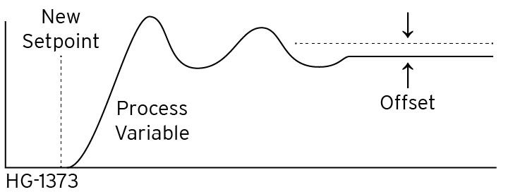
Proportional control often has an Offset factor. That is, the process almost never has 0 error. This can be caused by a variety of reasons, all of which are outside the realm of control of the Proportional function.

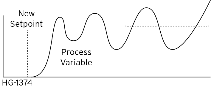
On the other hand, adding too much Proportional control can cause the process to oscillate and go further out of control:

Bias

If the offset in a process is constant, it can be removed by simply adding an equal-but-opposite value, called BIAS. This is a fixed value, which is determined by the user but is not changed or operated on by the PID control. Many processes can be effectively controlled using on Proportional control and a little bias.

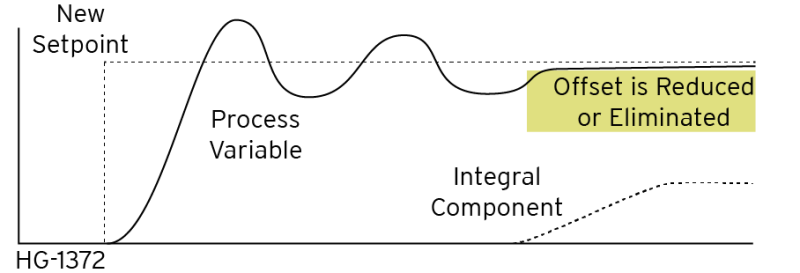
Integral Control

Integral functions are added to reduce the offset error amount. The Integral function works by measuring how long an error lasts and produces an additional error value that is added into the equation. This value is tuned such that it almost completely eliminates the Proportional Offset error.

The collecting and smoothing of values over time is known as integration. Because of the integrating action, the Integral portion of the control does not take full effect until the Process Variable starts to approach a steady-state (i.e., correction value become less and less significant) value. Quick changes in error are "smoothed out" by the integrating action, and have less effect on the process. As the Process Variable approaches steady-state, the Integral Error value becomes more important, and thus, serves to reduce the offset introduced by the Proportional control.

The problem with Integral control is that it does not respond well to quick changes in either the Setpoint or Process Variable. Although Integral control helps keep the process at a particular Setpoint, if either the Setpoint or Process Variable changes quickly, the Integral control has little effect.

Many processes respond well to Proportional-plus-Integral Control. In this case, Bias is reduced to 0 (zero).

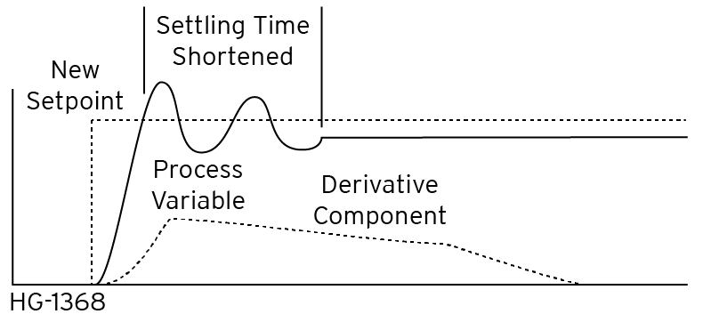
Derivative Control

The Derivative Control is introduced to handle quick changes in the process. The Derivative Control produces yet a third error signal based on the slope of the Error, or how much the error value changes in a given time period. When a change is first requested, the Error Slope is relatively steep and the Derivative portion of the error is significant. As the process reaches steady state the Error Slope will be shallow, and the effect of the Derivative control is reduced.

Return to the Top: PID in Advanced Ladder

Proportional-only Control

Proportional-only control is sufficient for a large number of processes, but neither Integral nor Derivative control alone is sufficient to control a process. Integral and Derivative are helpers, which respond to differing condition of the process. PID is an acronym for Proportional Integral Derivative. PID is a function that applies all three methods simultaneously in order to generate the controller output value. Not only is such a function concerned with the raw error (proportional), but it also considers how long the error has been in effect (integral) and how quickly the error value is changing (derivative).

When the process is first disrupted, the Proportional component attempts to make changes in the Controller Output. The Derivative aspect measures how great those changes are and adds a bit more of its value, thus making the controller act more aggressively to bring the process back to the setpoint. The Integral aspect has little effect here, because the error values vary greatly. As the process comes more into control, the magnitude of the Error begins to reduce. The Proportional component is still driving the process towards the setpoint, but with the change in errors becoming smaller and smaller, the Derivative component begins to be reduced. The Integral component, seeing that the error value is approaching a steady state value, begins to assert itself in order to reduce the errors due to offset.

Once the process reaches steady state, the Proportional component is producing very small error values and is attempting to produce some offset value. The Integral component measures how long the Error stays at one value, and produces its own error signal to compensate. Since the rate of change in Error is small, the Derivative component is almost non-existent. There are two common methods of implementing a PID function -- the Independent Method and the ISA Method.

Independent PID

CVout = (Kp * Error) + (Ki * Error * dt) + (Kd * Derivative) + CVBias

ISA PID

CVout = Kp * (Error + (Error * dt / Ti) + (Td * Derivative)) + CVBias

Where:

dt = Internal elapsed time clock - previous elapsed time clock

Derivative = (Error - previous Error)/dt

--or--

Derivative = (pv - previous PV)/dt

[User selectable during configuration].

Ti = Integral time

Td = Derivative time

The Independent PID is considered the standard. Although both methods provide the same results, the ISA PID is often easier to tune.

CVBias is an additive term separate from the PID components. This is most commonly used where only the Proportional (Kp) term is used (a proportional-only element). This forces CV Output to some non-zero value when the Process Variable (PV) is equal to the Setpoint (SP). CVBias is generally not used (set to 0) if the Integral term is used.

Tuning PID Loops

The object of a PID loop is, given a change in either the Setpoint SP or Process Variable PV, generate a Control Variable CV such that PV is driven towards and eventually stabilized at a value equal to the SP. This is done as rapidly as possible and with minimum fluctuations about the final value.

In order to meet these goals, the PID system must be tuned. That is, proper values must be selected for Kp, Ki, and Kd such that for any disruption in the process the process is returned to the desired value as quickly and as accurately as possible. These two requirements are usually mutually exclusive. A process can be controlled quickly but with less accuracy, or slower but more accurate. It is up to the process engineer to determine the optimal compromise between these two points, and make adjustment to the PID function (tune it) accordingly.

PID Tuning is considered difficult.

The users often use the "trial and error" method of tuning. Adjust the Kp, Ki, and Kd parameters and watch the process handle the next disturbance. If the control of the process is adequate, quit. Otherwise, tweak another control and try again. This process is time-consuming. An experienced process engineer usually has some feel for the process, and can make better estimates of the PID values. This is easier if the relationships among Kp, Ki, and Kd are understood.

Simply put, the Kp (proportional) control is the major factor in controlling the loop. Most loops can be brought into approximate control using Proportional only. The first step is to disable the Integral and Derivative controls and bring the process into alignment using only the Proportional Control. Using Proportional only usually results in an Offset Error. That is, the actual Process Variable value differs from the Setpoint value by a small, relatively constant amount. If the offset is small and remains constant, it can often be canceled using the CVBias value. Otherwise, set CVBias to 0 (zero) and try using Integral control.

The Ki (Integral) control was intended to reduce this error by adding an offset that is based on how long a specific error is present. The longer the error is present, the more effect the Integral control has. So with the Proportional Control properly set, begin to increase the Ki until the error is minimize, if not completely eliminated.

Most processes respond well to just these two adjustments, proportional and integral. However, one can find that the PV "wobbles" too much around the final value. This is known as a damped oscillation. Kp need to be adjusted just below the point that the process begins to oscillate and goes further out of control.

These oscillations can sometimes be further damped using the Kd (Derivative) control. The Derivative Control works on how fast the PV (and thus the resulting error) changes. The maximum rate of change occurs just after any disturbance, which is also when the Kp is oscillating. By increasing the Kd, the oscillations can be further damped to bring the process into control more quickly. PID tuning depends on the user's knowledge of the process to be controlled. Kp, Ki, and Kd are determined by the processes' characteristics, which must be understood before tuning can be performed.

There are two things that must be known about the process:

How big is the change in Process Value when Control Value is change by a fixed amount?
How quickly does Process Value change in response to a change in Control Value?

The change in PV is simply measured. When compared with CV using a simple equation, the OPEN LOOP GAIN (K) of the system is obtained:

Open Loop Gain (K) = PVstep / CVstep

If a step change in CV causes an identical step change in PV, the Open Loop Gain (K) is one (unity). If a step change in CV causes a step change in PV that is less than CV, the Open Loop Gain (K) is less than 1. If a small step change in CV causes a large change in PV, the Open Loop Gain (K) is greater than 1.

Most processes will not see any change in PV for some time after CV changes. This is called Pipeline Delay Time (Tp) or Dead Time. (Not to be confused with DEAD BAND.) The Time Constant (Tc) of the process is defined as the time between when the PV first starts to change and the time when PV reaches 63.2% of the expected final PV value.

Find K and Tc - Some experimenting must be done in order to obtain the desired values. This is best done by placing the PID Element into the MANUAL mode, make a small change in CV, and then plot the change in PV. For slow processes this can be done manually, but a strip chart recorder might be helpful. The change in CV is large enough to cause a measurable change in PV but not so large as to completely disrupt the process being controlled. The plot looks similar to the above graphic, and K, Tc, and Tp are easily measurable.

Ziegler-Nichols Tuning Method

Tune the Process

If K, Tc, and Tp are known we can use the following equations can be used to estimate starting values for Kp, Ki, and Kd in a Proportional / Integral / Derivative (PID) control:

Kp = (1.2 * Tc) / (K * Tp)

Ki = (0.6 * Tc) / (K * Tp * Tp)

Kd = (0.6 * Tc) / K

Tc and Tp are time units. It is important to ensure that both are expressed in identical units (i.e., milliseconds, seconds, hours, or whatever time frame is appropriate to the process). However, for use in the Cscape PID TUNE dialog, these values must be expressed 10mS intervals (eg: "100" = 10mS * 100 = 1 second).

If Proportional-only control (Ki and Kd = 0) is desired, use the equation:

Kp = Tc / (K * Tp)

Or for Proportional / Integral control (Kd = 0), use the equations:

Kp = 0.9 * Tc / (K * Tp)

Ki = 0.3 * Kp / T p

These equations are known as the Ziegler-Nichols tuning method, which were developed by John Zeigler and Nathaniel Nichols in the 1940's.

Return to the Top: PID in Advanced Ladder